
For systematic traders, the most practical starting point is an HMM-led pipeline validated with GMM or hierarchical clustering and retrained on a rolling walk-forward schedule. That combination gives you state continuity from the HMM, a soft-probability cross-check from the GMM, and a distribution-agnostic label anchor from clustering — all without requiring labeled training data you probably don't have.
The core evidence for this setup:
- HMMs produce more stable state sequences than k-means or GMMs alone, which matters when you're using regime labels to gate entries or size positions
- Hierarchical clustering on realized covariance matrices has shown the highest labeling accuracy in empirical tests, particularly for separating stress from normal periods
- Walk-forward retraining is non-negotiable: a model fit once on historical data will silently degrade as market structure shifts
Immediate next steps:
- Prepare daily log returns and a realized volatility series (at minimum) for your target instrument
- Install
hmmlearnandscikit-learn; run a 2-state Gaussian HMM as your baseline - Validate with a feed-forward loop before touching any strategy logic
- Cross-check state labels against at least one clustering method to catch fragmentation artifacts
Pro Tip: Before fitting any model, plot your feature distributions by calendar year. If the distribution shifts visibly across years, your in-sample fit is almost certainly overstating out-of-sample stability.
Table of Contents
- What data and features actually drive detection quality?
- How do the main detection algorithms compare?
- How do you evaluate a regime detector and build a trustworthy backtest?
- How do you apply detected regimes to actual trading logic?
- What are the most common failure modes and how do you avoid them?
- Why realized covariances and hierarchical clustering deserve a closer look
- Key Takeaways
- The gap between regime detection theory and what actually ships
- Disciplineaiapp brings regime-aware intelligence to your trading workflow
- Useful sources and further reading
What data and features actually drive detection quality?
Feature choice matters more than model choice in most cases. A well-engineered feature set fed to k-means will often outperform a poorly specified HMM.
Primary inputs worth including:
- Log returns (daily or higher frequency) as the baseline signal
- Realized volatility (RV), computed from intraday data when available, or from a rolling squared-return estimator on daily data
- Realized covariance matrices across a basket of assets, which embed macro-driven co-movement information that single-asset volatility misses
- Cross-sectional breadth measures (e.g., fraction of assets above their 200-day moving average) as a slow-moving macro signal
- Directional-change indicators as an alternative to time-based sampling, particularly useful for crypto markets with irregular volatility clustering
Frequency tradeoffs are real. High-frequency realized covariances aggregated to monthly labels give you cleaner regime boundaries but fewer training samples. Daily inputs give you more observations but noisier transitions. For most equity and crypto applications, daily features with a 21-day rolling window for volatility estimation is a reasonable starting point.
Feature transforms to apply before fitting:
- PCA or factor reduction on covariance matrices to reduce dimensionality before clustering
- Rolling z-scoring of each feature to remove slow drift from the input space
- Lagged features (t-1, t-5) to give sequential models a memory signal without requiring full recurrent architecture
Pro Tip: Avoid feeding raw price levels or cumulative returns as features. Models will learn the trend in your training window and produce regime labels that are really just "up period" vs. "down period" — which is not the same as a regime.
Label scarcity is the central challenge. Crash regimes might represent a small portion of your historical data, which means any supervised classifier will be class-imbalanced and prone to overfitting on the minority class. That's why most production pipelines use unsupervised methods and then validate pseudo-labels against known events (e.g., 2008, March 2020, the 2022 crypto drawdown) rather than training on labeled examples.
Data hygiene is unglamorous but consequential. Missing ticks, corporate actions, and timezone misalignment in intraday data will corrupt realized covariance estimates in ways that are hard to detect after the fact. Microstructure noise in high-frequency data inflates realized variance; a simple bias correction (e.g., the Newey-West adjustment or subsampling) is worth the effort before computing any covariance-based features.
How do the main detection algorithms compare?
Each method has a different core assumption, and that assumption determines where it succeeds and where it breaks.
Market regime detection using statistical and ML-based approaches demonstrates all three major families on S&P 500 futures with feed-forward retraining, and the practical differences are visible in the results.
Hidden Markov Models (HMM)
HMMs model the market as a latent state process where each state emits observations from a Gaussian (or mixture) distribution. The Viterbi algorithm decodes the most likely state sequence; the Baum-Welch algorithm (a special case of EM) estimates parameters. The key advantage is state continuity: the transition matrix penalizes rapid state switching, which produces more stable regime labels. The downside is sensitivity to initialization and the number of states, plus meaningful computational cost when retraining frequently on large feature sets.
Python: hmmlearn.hmm.GaussianHMM or pomegranate for more flexible emission distributions.
Gaussian Mixture Models (GMM)
GMMs cluster observations into K Gaussian components using EM-based soft assignment. Unlike HMMs, GMMs have no temporal structure — each observation is assigned independently. That makes them faster and easier to initialize, but it also means they can produce noisy, rapidly switching labels. The soft-probability output (posterior responsibilities) is genuinely useful: you can threshold at 0.7 or 0.8 to require high-confidence regime assignments before acting.
Python: sklearn.mixture.GaussianMixture with covariance_type='full' for most regime tasks.
K-means and agglomerative/hierarchical clustering
K-means partitions observations into K clusters by minimizing within-cluster variance. It's fast, interpretable, and a good baseline, but it assumes spherical clusters and has no temporal memory. Agglomerative clustering builds a dendrogram from pairwise distances, which is particularly useful when applied to realized covariance matrices: you're clustering covariance structures rather than return observations, and the dendrogram naturally reveals how many regimes are meaningfully distinct.
Python: sklearn.cluster.KMeans and sklearn.cluster.AgglomerativeClustering.
Change-point detection
Methods like PELT (via the ruptures package) or BOCPD detect abrupt structural breaks rather than persistent states. They're best for identifying when a regime changed rather than what regime you're in. Useful as a complement to HMM/GMM, not a replacement.
| Method | Detection accuracy | State continuity | Hyperparameter sensitivity | Computational cost | Interpretability | Out-of-sample robustness |
|---|---|---|---|---|---|---|
| HMM (Gaussian) | High for persistent regimes | High (transition matrix) | Moderate (n_states, init) | Moderate | Moderate | Good with walk-forward |
| GMM | Moderate | Low (no temporal structure) | Moderate (n_components, cov type) | Low | High | Moderate |
| K-means | Moderate | Low | Low (K only) | Very low | High | Moderate |
| Hierarchical clustering | High (covariance-driven) | Medium (post-hoc smoothing needed) | Low | Low–moderate | High | Good |
| Change-point (PELT) | High for abrupt shifts | N/A (event-based) | Moderate (penalty param) | Low | High | Good |
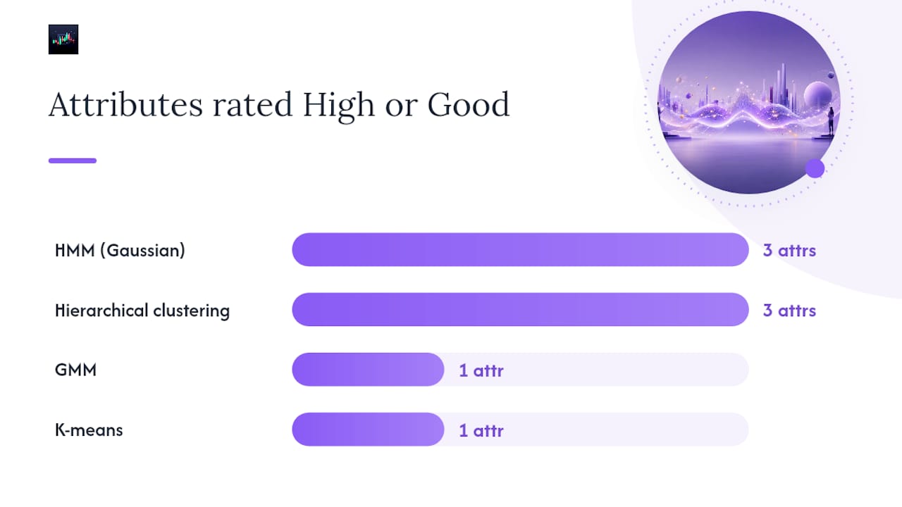
When to prefer clustering over sequential models: If your primary goal is labeling historical data for strategy research, hierarchical clustering on realized covariance factors is often the fastest path to high-quality labels. If you need real-time state assignment with low switching noise, HMM is the better choice. For production systems, a two-layer approach works well: cluster offline to generate reference labels, then train an HMM to reproduce those labels in real time.
For the number of states, two or three is almost always the right answer for a first implementation. More states increase the risk of fragmentation (short-lived micro-regimes that don't correspond to anything tradeable) and reduce the sample size per state.
How do you evaluate a regime detector and build a trustworthy backtest?
The biggest mistake in regime-detection backtesting is treating the regime labels as given and only evaluating the downstream strategy. You need to evaluate the detector itself first.
Evaluation metrics to report per model:
- State persistence: Average number of consecutive days in each state; short persistence (under 5 days) usually indicates fragmentation
- Precision/recall for crash detection: When labeled events exist (2008, March 2020), measure how often the model correctly flags them and how early
- Time-to-detect (lag): How many days after a known regime change does the model's state assignment flip?
- Conditional Sharpe and max drawdown: Strategy performance metrics computed separately for each detected regime
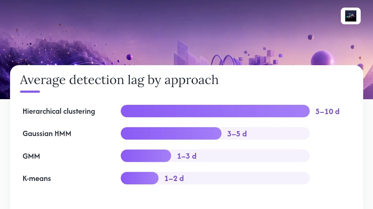
| Model | Detection accuracy | Avg state length (days) | Lag (days) | Conditional Sharpe (calm) | Conditional Sharpe (stress) |
|---|---|---|---|---|---|
| Gaussian HMM (2-state) | High | 20–40 | 3–5 | Report per backtest | Report per backtest |
| GMM (2-component) | Moderate | 5–10 | 1–3 | Report per backtest | Report per backtest |
| K-means (K=2) | Moderate | 5–12 | 1–2 | Report per backtest | Report per backtest |
| Hierarchical clustering | High | 15–30 | 5–10 | Report per backtest | Report per backtest |
The lag and average state length figures above are illustrative ranges drawn from published practitioner implementations; your actual numbers will depend on your feature set and retraining cadence.
Walk-forward validation structure:
- Training window: 252 days (1 year) minimum
- Out-of-sample test window: 63 days (1 quarter) per fold
- Warm-up period: 21 days at the start of each fold to allow the model to settle into a stable state
- Minimum folds: 8–10 to get a meaningful distribution of out-of-sample performance
Backtest caveats that actually matter:
- Transaction costs and slippage must be modeled explicitly. A regime filter that reduces trade count by 40% looks great on gross returns; on net returns after realistic costs, the improvement often shrinks significantly
- Lookahead leakage is easy to introduce when computing rolling features: make sure your feature at time t uses only data available at t, not t+1
- Confirmation rules (requiring N days in a state before acting) reduce false positives but introduce lag; test both versions and report the tradeoff
Tracking profit factor alongside Sharpe and drawdown gives you a cleaner picture of whether the regime filter is improving your edge or just reducing trade frequency.
How do you apply detected regimes to actual trading logic?
Regime labels are most useful as overlays, not as standalone signals. The goal is to improve the risk profile of an existing strategy, not to replace its entry logic.
Common application patterns:
- Conservative gating: Only take new entries when the regime detector signals "calm." Existing positions are held through regime transitions. This reduces trade count and drawdown without requiring you to exit at potentially bad prices.
- Protective gating: Exit open positions when the regime flips to "stress." More aggressive, more sensitive to detection lag, and more expensive in transaction costs.
- Position sizing multiplier: Scale position size by regime (e.g., 100% in calm, 50% in uncertain, 0% in stress). Smoother than binary gating and less sensitive to false positives.
- Multi-model consensus: Only act when at least two of your three detectors (HMM, GMM, hierarchical) agree on the state. Reduces false positives at the cost of some detection lag.
KPIs to monitor after deploying a regime filter:
- Trade count per regime (confirm the filter is actually gating entries as intended)
- Win rate and average R-multiple conditional on regime
- Drawdown reduction versus unfiltered baseline
- Filter flip frequency (high flip rate suggests fragmentation or overfitting)
Pro Tip: Layer regime filters on top of your existing risk manager rather than replacing it. If your strategy already has a max drawdown stop, the regime filter should reduce how often that stop gets hit, not substitute for it. Two independent risk controls are more robust than one.
Understanding how AI detects trading patterns at the feature level helps you design regime filters that complement rather than duplicate your existing signal logic.
What are the most common failure modes and how do you avoid them?
Most regime-detection failures fall into a small number of categories, and most of them are preventable.
Primary failure modes:
- Detection lag: The model correctly identifies a regime change but only after 5–10 days. By then, the damage to an unprotected position is done. Mitigation: use faster-updating features (shorter rolling windows, directional-change indicators) and accept slightly noisier labels.
- Label fragmentation: Too many states, or a model with no temporal memory, produces labels that flip every few days. Mitigation: enforce a minimum state-length filter; prefer HMM over GMM for real-time use.
- Overfitting to rare events: Crash regimes are rare. A model with 3+ states will often carve out a "crash" state that fits 2008 and 2020 perfectly in-sample but fires on noise out-of-sample. Mitigation: use 2 states for production; reserve 3+ states for research.
- Regime drift: Market structure changes over years. A model trained on 2010–2018 equity data will have miscalibrated transition probabilities for post-2020 crypto volatility. Mitigation: adaptive retraining cadence, triggered by distributional drift metrics (e.g., KL divergence between current feature distribution and training distribution).
- Lookahead leakage during retraining: If your retrain loop accidentally includes future data in the training window, your walk-forward results are meaningless. Mitigation: strict timestamp indexing; unit-test your data pipeline with a known-future data point and verify it's excluded.
Operational risks:
- Model serialization mismatches across library versions (see the pickle note above)
- Data pipeline breaks that silently feed stale or missing features to a live model
- Curve-fitting with small regime samples: if your "crash" state has fewer than 50 observations, treat any performance improvement with skepticism
Pro Tip: Build a real-time state-distribution dashboard that plots the rolling posterior probability of each regime. If the model starts assigning 90%+ probability to a single state for weeks at a time, it has likely drifted and needs retraining.
Why realized covariances and hierarchical clustering deserve a closer look
The most underused approach in practitioner pipelines is also one of the most empirically well-supported. Research on market regime detection via realized covariances shows that co-volatility information embedded in realized covariance matrices carries macro-driven regime signals that single-asset volatility measures miss. The study found that hierarchical clustering on covariance factors achieved the highest labeling accuracy in both simulations and empirical tests, with regime-switching models performing particularly well during stress periods.
The intuition is straightforward: when markets shift from calm to stress, it's not just that volatility rises — the correlation structure changes. Assets that were weakly correlated start moving together. That co-movement signal is invisible to a univariate volatility feature but clearly visible in a realized covariance matrix.
Implementation sketch:
- Compute realized covariance matrices at hourly frequency, then aggregate to monthly
- Extract the leading factors via PCA (typically 3–5 factors explain most variance)
- Cluster the monthly factor vectors using
AgglomerativeClusteringwith Ward linkage - Validate the resulting labels with an HMM or GMM to add temporal smoothing
- Back-test the labeled regimes against known macro events to sanity-check the labels
Statistical caveats: Stable covariance estimation requires a sample size substantially larger than the number of assets. For a 20-asset portfolio, you need at least 60–100 observations per estimation window; for 50 assets, consider shrinkage estimators (Ledoit-Wolf, available in sklearn.covariance) or factor models to regularize the matrix.
Key finding: Hierarchical clustering on realized covariance factors is distribution-agnostic and uses the full co-volatility information, which is why it tends to outperform simpler univariate approaches in empirical regime-labeling tasks.
| Approach | Detection accuracy | Avg lag (days) | Temporal smoothing needed | Best use case |
|---|---|---|---|---|
| Hierarchical clustering (covariance) | High | 5–10 | Yes (post-hoc) | Offline labeling, research |
| Gaussian HMM (returns + RV) | High | 3–5 | Built-in | Real-time filtering |
| GMM (returns + RV) | Moderate | 1–3 | Recommended | Soft-probability gating |
| K-means (returns only) | Moderate | 1–2 | Recommended | Baseline / fast prototype |
Advanced approaches worth tracking include deep learning state-space models (e.g., variational autoencoders for regime embeddings) and change-point methods from the recent statistical literature, though both require substantially more data and engineering overhead than the methods above.
Prediction market data is an emerging alternative signal source for macro regime indicators, particularly for event-driven regime shifts where traditional volatility measures lag the news.
Key Takeaways
An HMM-led pipeline with walk-forward retraining and hierarchical clustering for offline label validation gives systematic traders the best practical balance of accuracy, continuity, and out-of-sample robustness.
| Point | Details |
|---|---|
| Start with 2-state HMM | A 2-state Gaussian HMM with k-means initialization is the most stable baseline for real-time regime filtering. |
| Validate offline with clustering | Use hierarchical clustering on realized covariance matrices to generate reference labels before fitting any sequential model. |
| Walk-forward is mandatory | Fit once on historical data and your out-of-sample performance will be misleading; retrain on rolling windows of at least 252 days. |
| Lag vs. sparsity tradeoff | Faster features reduce lag but increase label noise; confirmation rules (3+ consecutive days) reduce noise but add lag. |
| Disciplineaiapp integration | Disciplineaiapp's multi-timeframe detection and confidence scoring provide a production-ready layer for applying regime signals to live trade filtering and position sizing. |
The gap between regime detection theory and what actually ships
Most articles on this topic treat regime detection as a modeling problem. It isn't, or at least that's not the hard part. The hard part is deploying a regime filter inside a live trading system and not letting it become a crutch for a strategy that was already marginal.
Here's what that means in practice: if your base strategy has a Sharpe of 0.4 unfiltered, a regime filter might push it to 0.6. That looks like a win. But you've now added a second model with its own parameters, its own retraining schedule, and its own failure modes. When the regime filter misfires during a fast-moving market, your strategy goes from underperforming to completely sidelined. That's a different kind of risk than the one you were trying to manage.
The right framing is to treat regime filters as risk overlays, not alpha generators. They should reduce the frequency and severity of drawdowns, not increase expected returns. If your regime filter is primarily improving returns rather than reducing drawdown, you're probably overfitting to the historical regime events in your training data.
The other thing practitioners consistently underestimate is retraining cadence. A model retrained annually on equity data will be badly miscalibrated for crypto volatility regimes, which can shift in days rather than months. The solution isn't to retrain daily — that introduces its own instability — but to monitor distributional drift continuously and trigger retraining when the feature distribution diverges meaningfully from the training distribution.
Disciplineaiapp's approach of continuously learning from market outcomes and evolving conditions is the right operational model: not a static detector, but a system that monitors its own calibration and adapts. That's harder to build than a one-time model fit, but it's the only version that holds up in production.
Disciplineaiapp brings regime-aware intelligence to your trading workflow
Most quant traders building regime detection pipelines spend weeks on model selection and almost no time on the operational layer: real-time state monitoring, confidence scoring, execution guidance, and trade journaling that ties regime context to actual outcomes.

Disciplineaiapp handles that operational layer. The platform's AI engine scans market structure, volatility conditions, and multi-timeframe alignment continuously, producing confidence-scored trade setups that already account for regime context. You get stand-aside protection when conditions are unfavorable, position sizing guidance calibrated to current volatility, and automated trade journaling that records the regime state at entry and exit — so your performance analytics show you exactly how your edge varies across market conditions.
For traders who want to go deeper, the AI Learning Center includes walkthroughs on regime-aware strategy construction and reproducible backtesting workflows. If you're ready to see the platform in action, the product overview covers the full feature set.
Useful sources and further reading
The libraries and papers below are the practical starting points for reproducing the pipelines described in this guide.
Libraries:
- Market regime detection via realized covariances
- Market regime detection using Statistical and ML based approaches
- scikit-learn.org
- cran.r-project.org
- en.wikipedia.org
- docs.python.org
- https://www.mdpi.com/1999-4893/11/12/202
- doi.org
Key papers and references:
- Realized covariances and hierarchical clustering for regime detection: The strongest empirical case for covariance-driven pipelines
- Practical HMM/GMM/clustering comparison on S&P 500 futures: Feed-forward implementation with strategy overlay examples
- HMMs applied to directional-change indicators: Cross-market regime profiling beyond volatility inputs
- Advanced statistical methods for regime detection: Change-point and state-space extensions for practitioners pushing beyond standard HMM/GMM
Reproducibility standards to follow: